Control System Analyzer: PID Tuning, Bode, Root Locus

Analyze a control loop from its transfer function, written the way it's written on paper. Type 10/(s^2 + 2s + 10), 2 e^(-3s)/(10s + 1) or G = 1/(s+1)^3; C = PID Kp=2 Ki=1 Kd=1. You get back:

• Stability, and the poles and zeros with their natural frequency, damping and time constant.
• The step response: rise time, settling time, overshoot, peak, final value, steady-state error and the peak control effort.
• Gain, phase and delay margins, the crossover frequencies, peak sensitivity Ms and bandwidth.
• Error constants (Kp, Kv, Ka) and the system type.
• A chart: the step response, the root locus (or pole-zero map), and the Bode magnitude and phase with the margins marked.

It also:

• Tunes P, PI and PID controllers with SIMC, AMIGO, IMC (lambda), Ziegler-Nichols, Cohen-Coon and an ITAE-optimal search. Every set of gains is tested on your real plant, compared side by side, and the best one is picked.
• Handles dead time exactly, in the margins and in the step response, not through a rough approximation.
• Turns a controller into code: the discrete transfer function and the difference equation, u[k] = 2.025·e[k] - 1.975·e[k-1] + u[k-1], ready for a microcontroller or PLC.
• Works in discrete time (z, with a sample time) as well as continuous time (s).

It's made for:

• Control and automation engineers tuning process loops.
• Robotics, motor-control and embedded developers.
• Students checking control-systems homework.
• AI agents that need real control math instead of rough guesses.

What it does

Writing systems

A transfer function can be:

• Text: numbers, s (or z), + - * / ^, parentheses and implicit multiplication. For example 5/(s(s+1)(s+5)), (s+2)/(s^2+0.4s+4), K/(tau s + 1) with params: {"K": 2, "tau": 5}, or G(s) = ....
• Dead time: e^(-3s), exp(-0.5s) or e^-2s.
• Coefficients: {"num": [1, 2], "den": [1, 3, 2]}, highest power first.
• Zeros, poles and gain: {"zeros": [-1], "poles": [-2, "-1+2j", "-1-2j"], "gain": 4}.
• State space: {"A": [[0, 1], [-2, -3]], "B": [[0], [1]], "C": [[1, 0]], "D": [[0]]}, with one input and one output.

Three modes

• A plant on its own: its poles and zeros, its own step response, its Bode plot and root locus, and the margins it would have under unity feedback.
• A closed loop: add a controller (PID gains such as PI Kp=1 Ti=5, a plain gain, or any transfer function), and optionally a sensor and positive feedback. You get the closed-loop poles, step response, control effort and the margins of the loop.
• Tuning: add tune and get gains from each rule. The plant is reduced to a first-order-plus-dead-time model (or an integrator plus dead time) for the rules. Then every set of gains is simulated on the real plant, with its overshoot, settling time, margins, Ms, ITAE and peak control effort. The pick is the lowest ITAE among the loops with a phase margin of at least 30° and overshoot within your limit.

Discrete controllers

Add discretize: {"dt": 0.01} and the controller is converted with Tustin's rule, or with ZOH, FOH, Euler, backward difference or pole-zero matching. You get the z-domain transfer function and the difference equation. Without a controller, the plant is discretized (ZOH by default), with dead time as whole samples.

Batches

Up to 500 systems per run, mixed freely.

How to use it

1. Write Systems, one per entry: a plant as text, or an object with plant, controller, tune and so on. The form has an example of each mode.
2. Set the Time unit if your model is in minutes or hours. Frequencies come out in rad per that unit.
3. Click Start. Each system is a row in the results, with its summary, chart and report.

Examples

All of these ran on this Actor, and the numbers are from the results.

System	Result
10/(s^2 + 2s + 10)	Stable, damping 0.316: 35.1% overshoot, settles in 3.54 s to 1. Under unity feedback it would have a 53.1° phase margin
5/(s(s+1)(s+5))	Has an integrator. Under unity feedback: gain margin 15.6 dB (6×), phase margin 43.2°, the same as MATLAB's margin
e^(-2s)/s	Under unity feedback: gain margin -2.1 dB and phase margin -24.6°, so the loop is unstable
G = 1/(s+1)^3; C = PID Kp=2 Ki=1 Kd=1	Closed loop stable: rise 1.58 s, settles in 7.82 s, 16.3% overshoot; gain margin 26.8 dB, phase margin 51.7°
{"plant": "1/(s+1)", "controller": "PI Kp=2 Ki=0.5", "discretize": {"dt": 0.1}}	u[k] = 2.025·e[k] - 1.975·e[k-1] + u[k-1]

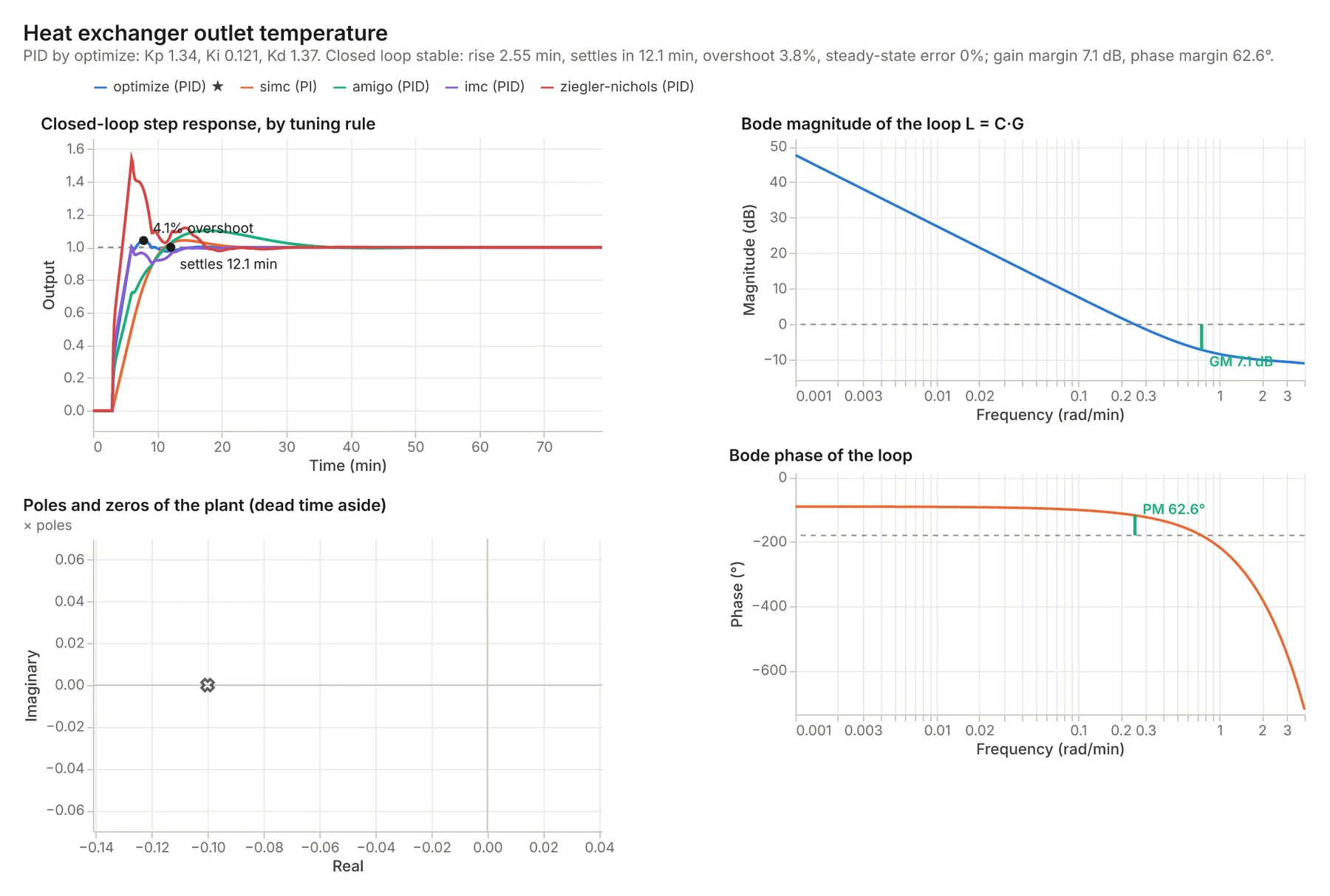
PID tuning for a heat exchanger (the picture above, in the form): 2 e^(-3s)/(10s + 1) in minutes.

Method	Kp	Ti (min)	Td (min)	Overshoot	Settling
SIMC (PI)	0.834	10.0		4.2%	18.2 min
AMIGO	0.850	6.90	1.38	10.1%	31.1 min
IMC	1.28	11.5	1.30	1.1%	13.3 min
Ziegler-Nichols	1.77	5.41	1.35	55.4%	20.1 min
ITAE search (picked)	1.34	11.1	1.02	3.8%	12.1 min

PID by optimize: Kp 1.34, Ki 0.121, Kd 1.37. Closed loop stable: rise 2.55 min, settles in 12.1 min, overshoot 3.8%, steady-state error 0%; gain margin 7.1 dB, phase margin 62.6°.

The numbers are checked in the tests:

• Second-order overshoot and peak time against the textbook formulas.
• Margins against python-control, and against a hand calculation for a dead-time plant.
• The exact dead-time response of a loop around e^(-s)/(s+1).
• Error constants.
• The model fit and the SIMC rule.
• Tustin's rule for a PI controller.

How-to examples

Each example is a complete input; the results are from runs of the Actor (also listed under Examples).

How to find the overshoot and settling time of a transfer function

{"systems": ["10/(s^2 + 2s + 10)"]}

Result: stable, damping 0.316, 35.1% overshoot, settling in 3.54 s to 1. Under unity feedback it would have a 53.1° phase margin. A step response, root locus and Bode plot come with it.

How to calculate gain and phase margins

{"systems": ["5/(s(s+1)(s+5))", "e^(-2s)/s"]}

Result: the first has a gain margin of 15.6 dB (6×) and a phase margin of 43.2°, the same as MATLAB's margin. The second, with 2 s of dead time, has a gain margin of -2.1 dB and a phase margin of -24.6°, so the loop is unstable. Dead time is handled exactly in the margins and the step response.

How to tune a PID controller

{"systems": ["2 e^(-3s)/(10s + 1)"], "timeUnit": "min"}

Result: SIMC, AMIGO, IMC, Ziegler-Nichols and an ITAE search are each tested on the plant and compared. The pick: "PID by optimize: Kp 1.34, Ki 0.121, Kd 1.37. Closed loop stable: rise 2.55 min, settles in 12.1 min, overshoot 3.8%, steady-state error 0%; gain margin 7.1 dB, phase margin 62.6°." Ziegler-Nichols, for comparison, overshoots by 55.4%.

How to let an AI agent analyze control loops

Add this Actor to the Apify MCP server with https://mcp.apify.com/?tools=jumblemog/control-systems-analyzer. The agent writes the transfer function as it's written on paper and passes on the margins, the step response numbers and tuned gains, instead of estimating them.

FAQ

How do I write the system? As on paper: 10/(s^2 + 2s + 10), 2 e^(-3s)/(10s + 1), or a plant and a controller such as G = 1/(s+1)^3; C = PID Kp=2 Ki=1 Kd=1. Discrete systems in z with a sample time work too.

Can it turn a controller into code? Yes. It gives the discrete transfer function and the difference equation, such as u[k] = 2.025·e[k] - 1.975·e[k-1] + u[k-1], for a microcontroller or PLC.

Are the results checked? Yes. The tests compare overshoot and peak time with the textbook formulas and the margins with python-control and a hand calculation.

Do I need MATLAB? No. It runs in the cloud, from the transfer function you type.

Does it work with Zapier, Make or n8n? Yes. Call the Actor with its Apify app or an HTTP request and pass the results on.

Input

Field	What it is
systems	Systems, as text or objects (see below).
params	Values for names used in every system's text, such as {"K": 2, "tau": 5}.
dt	Sample time for systems written in z.
timeUnit	s (default), min, h or any label.
charts	Draw charts (default on).

A system as an object takes these fields:

• plant: the system to analyze or control (required).
• controller: PID Kp=2 Ki=0.5 Kd=0.1, PI Kp=1 Ti=5, {"Kp": 2, "Ki": 1}, a number, or a transfer function. The derivative is filtered, Kd s/(Tf s + 1) with Tf = Kd/(N Kp), N = 10 by default (set N).
• sensor: the feedback-path transfer function.
• feedback: negative (default), positive, unity, or none for the open loop.
• tune: {"controller": "PI"} (P, PI or PID), methods (simc, amigo, imc, ziegler-nichols, cohen-coon, optimize, or all), tc (the closed-loop time constant for SIMC and IMC), maxOvershoot (%, default 10) and maxSensitivity (Ms, default 2). "tune": true tunes a PID.
• discretize: {"dt": 0.01, "method": "tustin"}.
• params, dt, timeUnit and title.

A line of text can hold a whole loop: G = 1/(s+1)^3; C = PID Kp=2 Ki=1 Kd=1; H = 1/(0.1s+1).

Output

One dataset item per system, also saved together in the run's OUTPUT record. A closed loop:

{
  "request": 3,
  "status": "ok",
  "mode": "closed-loop",
  "title": "DC motor speed with a PI controller",
  "summary": "Closed loop stable: rise 0.0989 s, settles in 0.775 s, overshoot 30.5%, steady-state error 0%; phase margin 38.7°.",
  "plant": {"text": "0.01 / (0.005 s^2 + 0.06 s + 0.1001)", "stable": true, "dcGain": 0.0999,
            "poles": [{"real": -9.998, "imag": 0, "naturalFrequency": 9.998, "damping": 1, "timeConstant": 0.1}, "..."]},
  "controller": {"text": "(100 s + 200) / (s)", "gains": {"form": "PI", "Kp": 100, "Ki": 200, "Ti": 0.5}},
  "openLoop": {"systemType": 1, "errorConstants": {"Kp": "infinite", "Kv": 19.98, "stepError": 0, "rampError": 0.05},
               "margins": {"gainMargin": null, "phaseMargin": 38.67, "gainCrossover": 12.5, "delayMargin": 0.054,
                           "peakSensitivity": 1.785}},
  "closedLoop": {"stable": true, "bandwidth": 19.99, "steadyStateError": 0,
                 "step": {"riseTime": 0.0989, "settlingTime": 0.775, "overshoot": 30.49, "peak": 1.305, "finalValue": 1},
                 "controlEffort": {"initial": 100, "peak": 101.0, "final": 10.01},
                 "poles": [{"real": -5, "imag": -13.23, "damping": 0.354}, "..."],
                 "stepResponse": [{"t": 0, "y": 0}, "..."]},
  "discrete": {"dt": 0.01, "method": "tustin", "transferFunction": "(101 z - 99) / (z - 1)",
               "differenceEquation": "u[k] = 101·e[k] - 99·e[k-1] + u[k-1]"},
  "imageUrl": "https://api.apify.com/v2/key-value-stores/.../records/003-....png",
  "markdownUrl": "https://api.apify.com/v2/key-value-stores/.../records/003-....md"
}

• A plant on its own has openLoopStep (metrics and points) in place of closedLoop.
• Tuning adds tuning: the fitted model, the picked method, and every method's gains with its overshoot, rise and settling time, margins, Ms, ITAE and peak control effort.
• Every result has a chart (imageUrl PNG and svgUrl), a Markdown report (markdownUrl), warnings (instability, small margins, Ms above 2, non-minimum-phase zeros) and notes.

A system that can't be computed has "status": "failed" and the reason in error, and isn't billed.

How it works

1. Text is read by a small parser of its own (no eval) into polynomials and a dead time.
2. Frequency responses are evaluated exactly, dead time included as e^(-jωθ). Margins are found on a fine grid and refined by root finding.
3. Step responses come from python-control. A loop with dead time is simulated with the dead time exact: a sample-delay buffer at a fine step, so there are none of the false wiggles a Padé approximation adds at the start. Closed-loop poles and bandwidth use an order-6 Padé approximation of dead time.
4. Tuning fits a first-order-plus-dead-time model from two points of the plant's step response (Smith's method), applies the rules, and runs a Nelder-Mead search on ITAE with penalties for overshoot and Ms.
5. Charts are drawn with Vega-Lite and rendered with vl-convert.

Pricing

You pay per result, at the prices shown on this page:

• One low price per system analyzed, with its chart and report.
• A higher price per system tuned, which compares up to six tuning methods on the real plant.

Systems that can't be computed are never charged. If you set a maximum cost per run, the Actor stops before a system that wouldn't fit.

Speed

An analysis takes a few hundredths of a second plus its chart, and tuning about a second. A run through the API answers in about 5 to 10 seconds, including the cloud container starting.

Tips and limits

• Linear, time-invariant systems with one input and one output. Saturation, rate limits and nonlinear plants aren't modeled. Check the peak control effort against what your actuator can do.
• Tuning works on stable plants and plants with one integrator. For unstable plants, give a controller and read the margins.
• Discrete-time systems can't be tuned directly. Tune the continuous plant and discretize the controller.
• Root loci are drawn for loops without dead time. With dead time, the chart shows the plant's poles and zeros instead.
• Limits: 500 systems per run. Charts are drawn for the first 100.

For AI agents and developers

This Actor works with the Apify MCP server, so AI agents can call it as a tool. Pass systems as plain text and read summary, openLoop.margins, closedLoop and tuning from the result. A direct API call that waits for the answer:

curl -X POST "https://api.apify.com/v2/acts/jumblemog~control-systems-analyzer/run-sync-get-dataset-items?token=YOUR_TOKEN" \
  -H "Content-Type: application/json" \
  -d '{"systems": ["5/(s(s+1)(s+5))", {"plant": "1.5 e^(-0.8s)/((4s+1)(s+1))", "tune": {"controller": "PI"}}]}'

run-sync instead returns the run's OUTPUT: the status, the counts and every result as JSON.

In Python, with the apify-client package:

from apify_client import ApifyClient

client = ApifyClient("YOUR_TOKEN")
run = client.actor("jumblemog/control-systems-analyzer").call(run_input={
    "systems": [{"plant": "K e^(-theta s)/(tau s + 1)", "params": {"K": 0.8, "theta": 4, "tau": 25},
                 "tune": {"controller": "PID", "methods": "all"}, "discretize": {"dt": 1}, "timeUnit": "s"}],
})
for item in client.dataset(run["defaultDatasetId"]).iterate_items():
    print(item["summary"], item["discrete"]["differenceEquation"])

Credits

• Control math: python-control (BSD-3-Clause) and SciPy (BSD-3-Clause).
• Charts: Vega-Lite and vl-convert (BSD-3-Clause), with the Inter font (SIL Open Font License).
• Methods:
  • Skogestad, S. (2003), Simple analytic rules for model reduction and PID controller tuning, Journal of Process Control 13(4), 291-309.
  • Åström, K. J. and Hägglund, T. (2004), Revisiting the Ziegler-Nichols step response method for PID control, Journal of Process Control 14(6), 635-650.
  • Rivera, D. E., Morari, M. and Skogestad, S. (1986), Internal model control: PID controller design, Ind. Eng. Chem. Process Des. Dev. 25(1), 252-265.
  • Ziegler, J. G. and Nichols, N. B. (1942), Optimum settings for automatic controllers, Trans. ASME 64, 759-768.
  • Cohen, G. H. and Coon, G. A. (1953), Theoretical consideration of retarded control, Trans. ASME 75, 827-834.
  • Smith, C. L. (1972), Digital Computer Process Control, Intext.