Pipe Flow Calculator: Pressure Drop, Pipe Sizing, Pumps

Work out pipe pressure drop the way you'd describe the pipe. Type water at 20 C, 200 gpm through 300 ft of 3 in sch 40 steel with 6 elbows and 2 gate valves, rise 20 ft. You get back:

• The total pressure drop, split into pipe friction, each fitting and the rise.
• The velocity, Reynolds number, flow regime and friction factor.
• The head loss and friction gradient, the outlet pressure and the pumping power.

It also handles:

• Finding the flow that a given pressure drop drives.
• Sizing a pipe: the smallest nominal size that meets velocity and pressure-drop limits.
• Gases, with compressible (isothermal) flow and a choked-flow check.
• Pumps: where a pump curve meets its system curve, with the efficiency, shaft power and NPSH available.
• Pipe networks: looped or branched, with reservoirs, tanks and pumps, solved for every flow and pressure.

Fluids come with their properties at the temperature and pressure you give, from CoolProp:

• Water and seawater.
• Ethylene and propylene glycol and brines.
• Air, nitrogen, natural gas, steam, CO₂ and refrigerants.
• Fuels and oils (diesel, gasoline, kerosene, crude, hydraulic oil ISO VG 32/46/68), from typical values.
• Any liquid you describe by its density and viscosity.

Pipes are named the way they're sold: 2 in sch 40, DN50, 3/4 in type L copper, 6 in PVC sch 80 or 4 in SDR 11 HDPE. Results come in SI or US units, each with a one-line summary.

It's made for:

• Plumbing, HVAC, fire-protection and process engineers.
• Irrigation and water-utility designers.
• Engineering students.
• Developers building calculators.
• AI agents that need real hydraulics instead of rough guesses.

What it does

Pipe runs

A run gives you the pressure drop broken into pipe friction, each kind of fitting and the change in elevation, with a bar chart of where the pressure goes. It also returns:

• Velocity, Reynolds number, flow regime (laminar, transitional or turbulent) and the Darcy friction factor.
• Head loss and the friction gradient per 100 m or 100 ft.
• The outlet pressure, when you give the inlet pressure.
• The hydraulic power.

A run can have segments in series: different sizes, lengths, fittings and rises. The sudden contractions and expansions between segments are added for you.

The three modes

• Flow given: you get the pressure drop.
• Pressure drop given (or the inlet and outlet pressures): you get the flow.
• Sizing (sizePipe): the smallest size of the same material and schedule that meets your limits. The default limits are 3 m/s (10 ft/s) and 4 ft per 100 ft for liquids, and 20 m/s with a 10% pressure drop for gases. The result shows the sizes on either side of the pick.

Fittings

Fittings are named and counted in plain words:

• Elbows: 90° standard or long radius, 45°, 180° return bends, mitered.
• Tees: flow through the run or the branch.
• Valves, open: gate, ball, globe, butterfly, plug, diaphragm and angle.
• Check valves: swing, lift and tilting-disc, plus foot valves.
• Entrances and exits, and strainers.
• Any fitting with its own K: strainer K = 2.

Loss coefficients come from the Darby 3-K method, which accounts for the Reynolds number and the size, so laminar flow of viscous oils comes out right.

Gases

Compressed air, natural gas, steam and other gases use the isothermal compressible-flow equation, which stays accurate when the pressure drops a lot. Flows can be given as scfm, Nm³/h, MMSCFD, actual m³/h or kg/s. If the gas would reach its limiting velocity before the outlet, the result says the flow is choked. Finding the flow from a pressure drop works for gases too.

Pump systems

A pump system takes:

• The pump curve, from a few catalog points.
• Optionally, its efficiency and NPSH-required curves.
• The static head.
• The suction and discharge pipes.

It returns the operating point (flow, head, efficiency, shaft power), the NPSH available with a cavitation check, and the best-efficiency point. Pumps can run at another speed (affinity laws), or two or more can run in parallel or in series. Without a pump, it returns the system curve alone. The chart shows the pump curve, the system curve and the efficiency.

Networks

A network has junctions with demands, reservoirs and tanks at fixed heads, pipes (with fittings and check valves) and pumps. It is solved with Darcy-Weisbach or Hazen-Williams, using Newton's method on the whole network (the global gradient method that EPANET uses). You get:

• Every pipe's flow, direction, velocity and head loss.
• Every node's head and pressure.
• A drawing of the network: give nodes x and y coordinates, or it lays them out itself.

Batches

Up to 500 requests per run, mixed freely.

Who it's for

• Plumbing, HVAC and fire-protection designers: size water, chilled-water, glycol and compressed-air piping, and check pump selections.
• Process and mechanical engineers: pressure drop of oils, fuels, steam and gases through real fittings, and line sizing.
• Water and irrigation engineers: looped distribution networks with Hazen-Williams, pump operating points and NPSH.
• Students: check Moody-chart, Darcy-Weisbach and pump-curve homework, with every intermediate number shown.
• Developers and AI agents: a hydraulics API that takes plain sentences or JSON and returns exact numbers with their units.

How to use it

1. Write Pipe runs, one per line, such as water at 60 F, 150 gpm through 500 ft of 3 in sch 40 steel, 8 elbows, 1 check valve. Objects work too.
2. Add Pump systems or Pipe networks as JSON if you want them. The form has an example of each.
3. Leave Units on automatic (US units are picked when you write gpm, ft or psi), or choose SI or US.
4. Click Start. Each request is a row in the results, with its summary, chart and report.

Examples

All of these ran on this Actor, and the numbers are from the results.

Request	Result
water at 20 C, 200 gpm through 300 ft of 3 in sch 40 steel with 6 elbows, 2 gate valves and 1 check valve, rise 20 ft	22.19 psi in total: 11.4 psi pipe friction, 2.14 psi fittings, 8.66 psi for the rise; 8.68 ft/s, Re 205,485, f = 0.0192
compressed air at 7 barg and 25 C, 300 scfm through 150 m of DN50 galvanized pipe, 4 elbows	27.1 kPa drop, outlet 774.2 kPa abs; 482 Nm³/h, 8.53 m/s at the inlet
natural gas at 60 psig, 50 F, 1 mmscfd, 5 mi of 4 in sch 40	25.8 psi drop, outlet 48.9 psia (isothermal flow)
water 15 C, 3 in PVC sch 80, 100 m, available 2 bar	Flow 68.54 m³/h at 4.47 m/s, with a warning that the velocity is high
hydraulic oil ISO VG 46, 40 l/min, 5 m of ID 16 mm	Laminar (Re 1,153): 82.9 kPa, matching Hagen-Poiseuille
{"fluid": "ethylene glycol 30%", "temperature": "5 C", "flow": "30 m3/h", "material": "PVC", "length": "80 m", "sizePipe": true}	4 in sch 40 PVC (3 in would run at 4.4 ft per 100 ft): 1.02 m/s, 11.5 kPa

A booster pump (in the form): a pump curve from 160 ft at shutoff to 80 ft at 400 gpm, 85 ft of static head, a 5 in suction line and 600 ft of 4 in discharge with fittings.

Operating point: 287.9 gpm at 118.5 ft (51.32 psi), 74.9% efficient, 11.5 hp shaft power; static head 85 ft; NPSH available 36.73 ft vs 9.637 ft required.

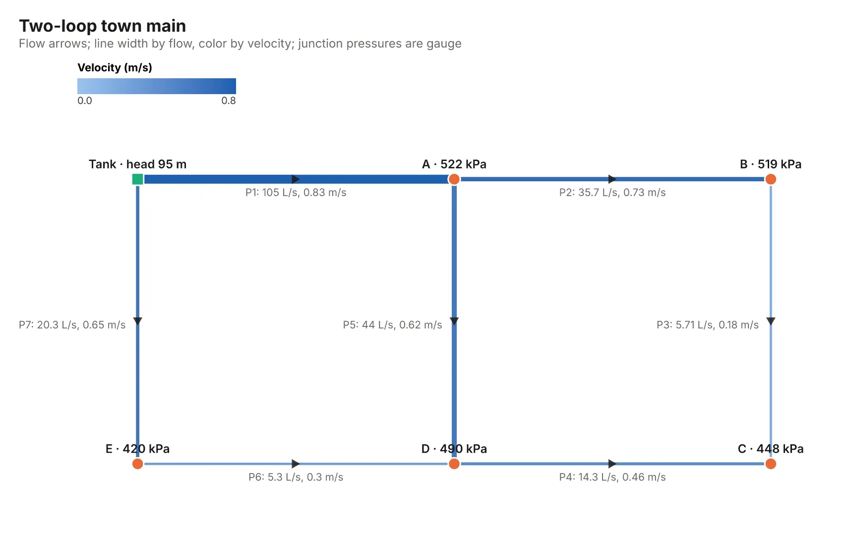
A two-loop town main (the picture above): a tank at 95 m head, five junctions with 125 L/s of demand and seven pipes, solved with Hazen-Williams C = 130.

6 nodes, 7 pipes and pumps, solved in 4 iterations (Hazen-Williams). Total demand 125 L/s; junction pressures from 419.6 kPa (E) to 522 kPa (A) gauge; fastest pipe P1 at 0.8332 m/s.

The numbers are checked against hand calculations in the tests:

• Darcy-Weisbach for turbulent water.
• Hagen-Poiseuille for laminar oil.
• The isothermal gas-flow equation.
• Hazen-Williams for a single main.
• A three-reservoir problem: flow balance at the junction, and the head loss across every pipe.

How-to examples

Each example is a complete input; the results are from runs of the Actor (also listed under Examples).

How to calculate pressure drop in a water pipe

{"pipes": ["water at 20 C, 200 gpm through 300 ft of 3 in sch 40 steel with 6 elbows, 2 gate valves and 1 check valve, rise 20 ft"]}

Result: 22.19 psi in total: 11.4 psi of pipe friction, 2.14 psi for the fittings and 8.66 psi for the rise, at 8.68 ft/s, Re 205,485 and f = 0.0192.

How to size a pipe for a flow

{"pipes": [{"fluid": "ethylene glycol 30%", "temperature": "5 C", "flow": "30 m3/h", "material": "PVC", "length": "80 m", "sizePipe": true}]}

Result: 4 in sch 40 PVC at 1.02 m/s and 11.5 kPa (3 in would lose 4.4 ft per 100 ft). Give an available pressure instead of a flow and it finds the flow: water 15 C, 3 in PVC sch 80, 100 m, available 2 bar gives 68.54 m³/h, with a warning that the velocity is high.

How to find a pump's operating point and NPSH

Give the pump curve and the piping in pumpSystems, as in the booster pump example in the input form. Result: "Operating point: 287.9 gpm at 118.5 ft (51.32 psi), 74.9% efficient, 11.5 hp shaft power; static head 85 ft; NPSH available 36.73 ft vs 9.637 ft required."

How to let an AI agent do pipe flow calculations

Add this Actor to the Apify MCP server with https://mcp.apify.com/?tools=jumblemog/pipe-flow-calculator. The agent describes the pipe the way an engineer would and passes on the pressure drop, velocity and warnings, with fluid properties at the real temperature instead of rough values.

FAQ

Which fluids does it know? Water and seawater, ethylene and propylene glycol and brines, fuels and hydraulic oils, compressed air, natural gas and other gases, with properties at your temperature and pressure (from CoolProp, or typical values for fuels and oils).

Which friction method does it use? Darcy-Weisbach with the Darcy friction factor, and the Darby 3-K method for fittings, which accounts for the Reynolds number and the size. Networks can use Hazen-Williams instead.

Does it handle gases? Yes, as compressible isothermal flow with a choked-flow check.

Can it solve a pipe network? Yes: looped or branched networks with reservoirs, tanks and pumps, solved for every flow and pressure.

Does it work with Zapier, Make or n8n? Yes. Call the Actor with its Apify app or an HTTP request and pass the results on.

Input

Field	What it is
pipes	Pipe runs, as text lines or objects (see below).
pumpSystems	Objects: pump (curve, efficiency, npshr, speed, count, arrangement), staticHead (or sourceElevation, destinationElevation, sourcePressure, destinationPressure), suction (pipe, length, fittings, liquidLevel above the pump, pressure), discharge (a pipe run), maxFlow (system curve alone).
networks	Objects: nodes (id, type reservoir or tank with head, level or pressure; junctions with elevation and demand; optional x, y), pipes (id, from, to, length, diameter or pipe, material, C, roughness, fittings, K, checkValve), pumps (id, from, to, curve), headloss (darcy-weisbach or hazen-williams).
fluid, temperature, pressure	Defaults for requests that don't give them (water at 20 °C if nothing is given).
units	auto (default), SI or US.
charts	Draw charts (default on).

A pipe run as an object takes these fields:

• Fluid: fluid, temperature, pressure (the inlet pressure, absolute or gauge; needed for gases), density or sg, and viscosity (cP or cSt).
• Flow: flow (volume, mass or standard flow) or velocity.
• Pipe: pipe (nominal size and schedule) or diameter (inside), material, roughness, length, fittings, K (extra losses) and rise (outlet elevation minus inlet).
• Mode: pressureDrop or outletPressure to find the flow; sizePipe, maxVelocity and maxPressureDrop (4 ft/100 ft, 2 psi/100 ft, 0.5 bar/100 m or a total) to size.
• Series: segments, a list of pipes each with its own pipe, length, fittings, K and rise.

Pipes it knows:

• Steel and stainless pipe in schedules 5 to 160, STD, XS, XXS, 5S, 10S, 40S and 80S, by NPS or DN.
• PVC and CPVC in schedules 40, 80 and 120, and PVC SDR pipe.
• HDPE SDR 7 to 32.5 (IPS sizes).
• Copper tube types K, L and M (ASTM B88).
• Any inside diameter.

Materials set the roughness and Hazen-Williams C: commercial steel, stainless, galvanized, corroded steel, cast iron, ductile iron, copper, PVC, CPVC, ABS, HDPE, PEX, fiberglass, concrete and more. You can give your own roughness or C.

Units it reads:

• Flow: gpm, l/s, l/min, m³/h, m³/s, cfm, cfs, bbl/day, MGD.
• Mass flow: kg/s, kg/h, t/h, lb/h.
• Standard gas flow: scfm, scfh, MMSCFD, Nm³/h, Sm³/h, slpm.
• Pressure: Pa, kPa, MPa, bar, psi, psig, barg, atm, inH₂O, mmHg.
• Head: m, ft.
• Length and diameter: m, mm, km, ft, in, mi.
• Velocity: m/s, ft/s.
• Viscosity: cP, Pa·s, cSt.
• Density: kg/m³, lb/ft³, SG.
• Temperature: C, F, K.

Output

One dataset item per request, also saved together in the run's OUTPUT record. A pipe run:

{
  "request": 1,
  "status": "ok",
  "type": "pipe",
  "mode": "drop",
  "title": "Pressure drop: Water in 4 in sch 40 commercial steel",
  "summary": "Water at 20 °C, 54 m³/h through 250 m of 4 in sch 40 commercial steel: 198.4 kPa total pressure drop (75.89 kPa pipe friction, 5.035 kPa fittings, 117.5 kPa to lift it); velocity 1.826 m/s, Re 186,219 (turbulent), friction factor 0.0186. Outlet pressure 502.9 kPa abs.",
  "fluid": {"name": "Water", "phase": "liquid", "temperature": 20.0, "density": 998.482, "viscosity": 1.00141, "vaporPressure": 2.33932},
  "results": {
    "pressureDrop": 198.425, "frictionLoss": 75.8882, "fittingsLoss": 5.03548, "elevationChange": 117.501,
    "headLoss": 8.26446, "velocity": 1.82637, "reynolds": 186219, "regime": "turbulent", "frictionFactor": 0.01864,
    "frictionGradient": 30.3553, "outletPressure": 502.9, "hydraulicPower": 2.97637
  },
  "segments": [{
    "pipe": "4 in sch 40 commercial steel (ID 4.026 in, 102.3 mm)", "insideDiameter": 102.26,
    "fittings": [{"fitting": "90° elbow", "count": 4, "K": 0.3354, "loss": 2.23446},
                 {"fitting": "Swing check valve", "count": 1, "K": 1.682, "loss": 2.80102}]
  }],
  "unitLabels": {"pressureDrop": "kPa", "velocity": "m/s", "frictionGradient": "kPa/100 m", "...": "..."},
  "imageUrl": "https://api.apify.com/v2/key-value-stores/.../records/001-....png",
  "markdownUrl": "https://api.apify.com/v2/key-value-stores/.../records/001-....md"
}

The other request types add their own fields:

• Sized runs add sizing: the limits, the size chosen, and the sizes tried with their velocity and pressure drop.
• Pump systems have operatingPoint and curve (system head, pump head and efficiency by flow).
• Networks have pipes and nodes, with csvUrl for both as CSV.
• Every result has a Markdown report (markdownUrl), warnings (high velocity, cavitation, choked flow, low NPSH margin, negative pressures) and notes (assumptions such as a schedule or temperature that wasn't given).

A request that can't be computed has "status": "failed" and the reason in error, and isn't billed.

How it works

1. Each request is read into a fluid, a flow and pipe segments in SI units. Text lines are split into phrases, and each phrase is recognized by its units and words.
2. Fluid properties come from CoolProp: reference equations of state for pure fluids, and incompressible fits for glycols, brines and seawater.
3. Pipe dimensions come from the ASME B36.10M/B36.19M, ASTM D1785, F441, F2619 and B88 tables (through the fluids library), and the friction factor from the Colebrook equation, solved exactly. Laminar flow uses 64/Re.
4. Gas runs are solved segment by segment with the isothermal flow equation, P₁² − P₂² = G²(P₁/ρ₁)(fL/D + ΣK + 2 ln P₁/P₂). Flows from pressure drops and sizing use the same model inside a root finder.
5. Networks are solved by Newton's method on all flows and heads at once, with a line search. Check valves and pumps resist reverse flow.
6. Charts are drawn with Vega-Lite and rendered with vl-convert.

Pricing

You pay per result, at the prices shown on this page:

• One low price per pipe run, whether it computes the pressure drop, finds the flow or sizes the pipe.
• A higher price per pump system or network, with its chart, report and tables included.

Requests that can't be computed are never charged. If you set a maximum cost per run, the Actor stops before a request that wouldn't fit.

Speed

A pipe run takes a few milliseconds plus its chart, and a network of a few hundred pipes solves in about a second. A run through the API answers in about 5 to 10 seconds, including the cloud container starting.

Tips and limits

• Single-phase flow only: boiling liquids and two-phase steam-water flow aren't covered. A liquid whose outlet pressure falls below its vapor pressure gets a cavitation warning.
• Hot water needs its pressure: water above 100 °C is steam at 1 atm, so give the pressure in the pipe.
• Oils and fuels from the built-in list use typical values that don't change with temperature. Give density and viscosity for your product and temperature.
• Transitional flow (Re 2,000 to 4,000) uses the turbulent friction factor, which is the conservative choice, and says so.
• Gas networks aren't covered. Compute gas lines as pipe runs.
• Limits: 500 requests per run, 100 segments per run, 1,000 nodes and 2,000 pipes and pumps per network.

For AI agents and developers

This Actor works with the Apify MCP server, so AI agents can call it as a tool. Pass pipes as plain sentences and read summary and results from the result. A direct API call that waits for the answer:

curl -X POST "https://api.apify.com/v2/acts/jumblemog~pipe-flow-calculator/run-sync-get-dataset-items?token=YOUR_TOKEN" \
  -H "Content-Type: application/json" \
  -d '{"pipes": ["water at 60 F, 150 gpm through 500 ft of 3 in sch 40 steel, 8 elbows, 1 check valve", "compressed air at 100 psig, 200 scfm, 300 ft of 1-1/2 in sch 40"]}'

run-sync instead returns the run's OUTPUT: the status, the counts and every result as JSON.

In Python, with the apify-client package:

from apify_client import ApifyClient

client = ApifyClient("YOUR_TOKEN")
run = client.actor("jumblemog/pipe-flow-calculator").call(run_input={
    "pipes": [{"fluid": "water", "flow": "40 l/s", "material": "ductile iron", "length": "800 m",
               "sizePipe": True, "maxVelocity": "1.5 m/s"}],
    "pumpSystems": [{"pump": {"curve": [["0 m3/h", "45 m"], ["60 m3/h", "40 m"], ["120 m3/h", "28 m"]]},
                     "staticHead": "18 m", "discharge": "400 m of DN150, 6 elbows, 1 check valve"}],
})
for item in client.dataset(run["defaultDatasetId"]).iterate_items():
    print(item["summary"])

Credits

• Pipe dimensions, friction factors and fitting coefficients: fluids by Caleb Bell (MIT).
• Fluid properties: CoolProp by Ian Bell and contributors (MIT).
• Network layout: NetworkX (BSD-3-Clause).
• Charts: Vega-Lite and vl-convert (BSD-3-Clause), with the Inter font (SIL Open Font License).
• Methods:
  • Darby, R. (2001), Correlate pressure drops through fittings, Chemical Engineering 108(7), 127-130.
  • Crane Co., Flow of Fluids Through Valves, Fittings, and Pipe, Technical Paper 410.
  • Clamond, D. (2009), Efficient resolution of the Colebrook equation, Ind. Eng. Chem. Res. 48(7), 3665-3671.
  • Todini, E. and Pilati, S. (1988), A gradient algorithm for the analysis of pipe networks.